Lines and loops.

In many cases, three-dimensional and flat primitives are not enough to build the required geometry. Advanced operations, from among those that are found in this tutorial, allow you to create geometric bodies based on arbitrary lines.

In ZenCad (and the opencascade geometric kernel), there are two classes of one-dimensional geometric solids - Edge and Wire. Edge is a simple primitive. Combining multiple Edges into a single compound curve results in a Wire object. Typically, ZenCad, Wire, and Edge can be used interchangeably, but when analyzing a model using reflection, this difference can be significant. ")

The Wire and / or Edge set can be connected to a complex curve using the sew function (More details later in this section).

Closed curves are called cycles. If the curve (all compound curves) of the cycle lies in the same plane, then such a cycle can be converted into a face (Face) using the fill function (see the section "Plane primitives".).

Some additional operations when working with curves are described in the "Curve Analysis" section.

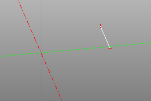
Segment

An ordinary segment, specified by two points.

Signature:

segment(pnt1, pnt2)

Polysegment

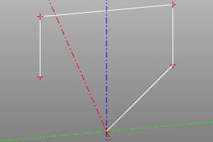
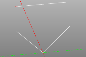
Polysegment is a broken line. Set by an array of points. Setting the closed flag adds a polyline segment from the end point to the start point. pnts is an array of points.

Signature:

polysegment(pnts, closed=True/False)

Point Interpolation

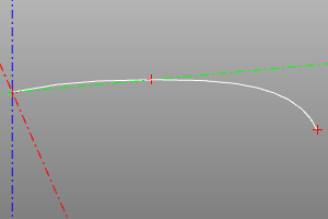
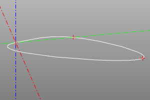
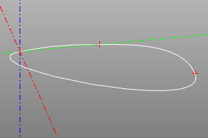
Tool for constructing an interpolated curve passing through a set of pnts points. Using the optional tangs parameter at each point, you can set the direction in which the curve will pass through the point (the zero vector corresponds to an arbitrary intersection). Setting the closed flag adds a trailing portion of the curve.

Signature:

interpolate(pnts, tangs=[], closed=False)

Arc of a circle with three points

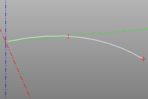
This method represents an alternative to circle (see Plane Primitives) method of generating a circular arc from three points.

Signature:

circle_arc(p1, p2, p3)

Upward spiral

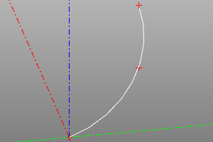
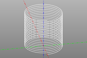
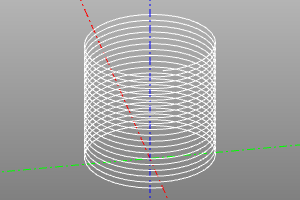
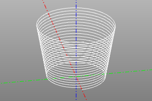
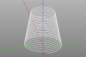
An upward spiral. It is set by the radius r, the height h and the step of the loop step. When setting the option left, it changes the right winding to the left one. When setting the optional parameter angle, the radius changes with the change of height according to the conical law.

Signature:

helix(r, h, step, angle=angle, left=True/False)

Bezier Curve

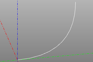
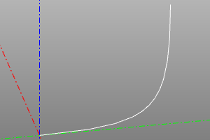
Bezier curve (wiki). Defined by an array of control points and an array of weights (optional). If weights are not specified, all weights are considered equal to one.

Signature:

bezier(pnts)
bezier(pnts, weights)

BSpline

Signature:

bspline(pnts, knots, muls, degree, periodic=False/True)
bspline(pnts, knots, weights, muls, degree, periodic=False/True, check_rational=False/True)

default:
periodic=False
check_rational=True

Rounded polysegment

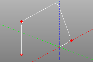
Unlike a polysegment, it creates sections of a circle at the mating points of the segments. The r variable sets the radius of the fillets. Can be used in conjunction with the tube operation (see kinematic surfaces). The closed option allows you to close the curve and create a rounded segment at the junction.

Signature:

rounded_polysegment(pnts, r, closed=False)

Example:

rounded_polysegment(
pnts=[(0,0,0), (20,0,0), (20,20,40), (-40,20,40), (-40,20,0)],
r=10)

Creating a complex curve

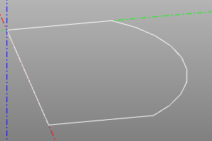
The sew operation assembles a complex line from an array of wires pieces.

Objects of types Edge and Wire can act as elements of the wires array (see geometric types)

Requirements. Parts of the line must necessarily border on each other. The order should not be out of order. If the sort argument is set, the algorithm will try to automatically sort the incoming lines in the correct order.

Signature:

sew(wires, [sort=True])

Example:

sew([
segment((0,0,0), (0,10,0)),
circle_arc((0,10,0),(10,15,0),(20,10,0)),
segment((20,0,0), (20,10,0)),
segment((20,0,0), (0,0,0))
])

Complex curve constructor

Tool for sequential construction of curve sections. Performing operations, constructs edges from the exit point of the previous edge. Each operation can be performed in absolute and relative modes. In relative mode, the coordinates of the anchor points are added to the last current coordinate of the constructor. The choice of the mode is carried out by the rel flag. False is absolute, True is relative. If no flag is declared, the defrel value is used.

Constructor arguments: start - starting point defrel - default mode

wb = wire_builder(start=(0,0,0), defrel=False)

Reinitialization:

Reloads the instrument from a new point. Resets the list of edges.

wb.restart(pnt, y=None, z=None)

wb.restart(point3(10,15,0))
wb.restart(10,15)

Drawing a line segment:

Draws a segment to the point pnt.

wb.segment(pnt, y=None, z=None, rel=None)
wb.line(b, y=None, z=None, rel=None)
wb.l(b, y=None, z=None, rel=None)

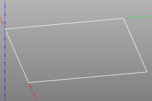
wire_builder(defrel=True).restart((0,10)).l(10,0).l(0,-10).close().doit() # рисуем квадрат

Draw a circular arc by points:

wb.arc_by_points(a,b,rel=None)

Plotting an interpolation curve by points:

curtang allows you to set the direction of the curve at the starting point. Setting the approx option calculates curtang to the direction of the curve at the end of the last leg.

wb.interpolate(pnts, tangs=None, curtang=(0,0,0), approx=False, rel=None)

Closure

close builds a section of the curve up to the starting point. approx_a, approx_b allow for interpolation at snapping points.

wb.close(approx_a=False, approx_b=False)